To understand the power of the GEKO turbulence model, we must first answer the following question – “What is special about the GEKO model compared with all other two equation RANS models?” The GEKO model is based on the Shear Stress Transport (SST) model which combines the best of the k-ω and k– ε models and a shear stress realizability criterion [1]. The GEKO model is the result of the decades of experience that Dr. Florian Menter has acquired through his vast experience of turbulence modelling at NASA and Ansys. It is very much the culmination of a life’s work on improving turbulence models to make them what he calls “industrial strength”.
So, we are off to a good start! What sets the GEKO model apart is the way the various model constants are specified, allowing control of a single physics by a single constant. For example, C(sep) controls boundary layer separation from smooth surfaces, C(mix) controls mixing in free shear layers, and so forth [2]. Experimental data can be used to tune the GEKO constants, and then these “optimised” constants can be used confidently for future simulations.
Next question, “Why would you bother to do this?” Often there is no need to tune a model if a Scale Resolving Simulation is performed using an advanced approach such as SBES [3]. However, such simulations are always going to require fine meshes, lots of small timesteps and therefore significant run times and computing resources. On the other hand, the GEKO model permits a much-reduced mesh size and can generally be run steady-state. (In fact, running GEKO, or any other two equation model, transiently requires extra care to ensure you are not predicting unphysical turbulence – if you are intending to do this, we strongly recommend you review this reference [4]).
The remainder of this blog is devoted to work arising from a recent collaboration between staff at Deakin University, RMIT and The University of Sydney which demonstrates the successful application of GEKO turbulence model to a real-world application. The work addresses the modelling of flow through a stenosis, a geometry of great significance in biomedical flows. The publication was selected for the cover article of the open access journal fluids (shown below). As it is open access you can download if freely at https://doi.org/10.3390/fluids10070168 [5].
The work in the paper compares simulations of flow though stenoses ranging from 25-75% and compares the results with previously published work. Some key points arise from the work:
- The default blending function between the two RANS models does not work well in this internal flow and was overridden using a UDF to ensure the k-ω model is applied only in the near wall region.
- The simulations were at a relatively low Reynolds number of 2,000 which classically would be considered as leading to laminar flow, but upstream disturbance trigger turbulence-like behaviour at this low Reynolds number (in a range directly relevant to biomedical flows).
- The results are affected by the upstream turbulence intensity if it is above a threshold of approximately 1%.
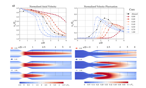
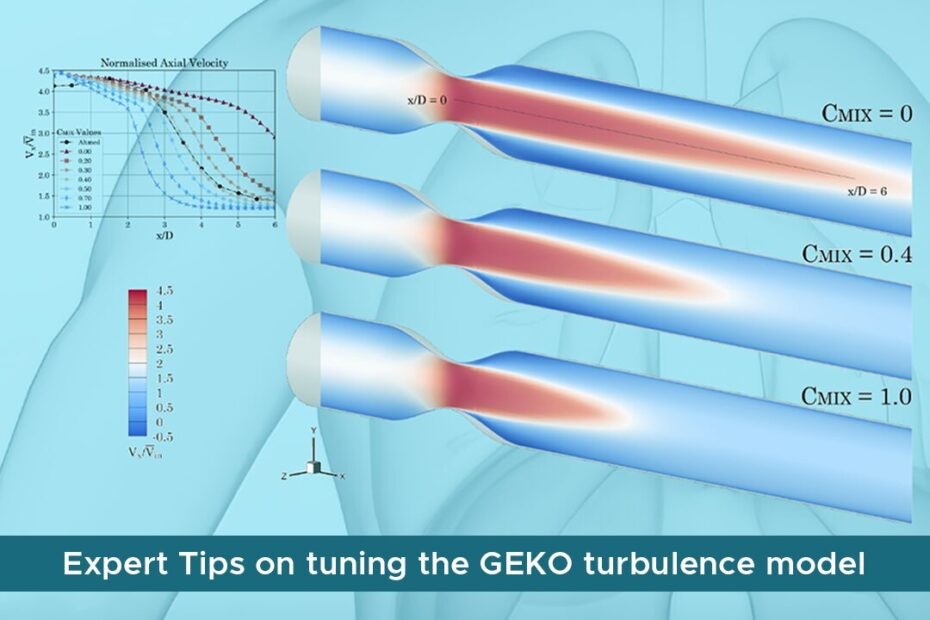
- The parameter C(mix) proved to be the most important by far and a value of 0.4 (increased from a default of 0.3) gave good agreement with the experimental data. Its effect is shown below in Fig. 2.

Fig. 2 Results for a range of C(mix) values for Re = 2000 plotted against the experimental data of Ahmed and Giddens [6]. (a) Plots of normalised axial velocity and velocity fluctuations along the centreline. Contours of normalised axial velocity and velocity fluctuations plotted on the centre plane for a range of C(mix) values are also shown to highlight its effect on the flow field. Taken from [5].
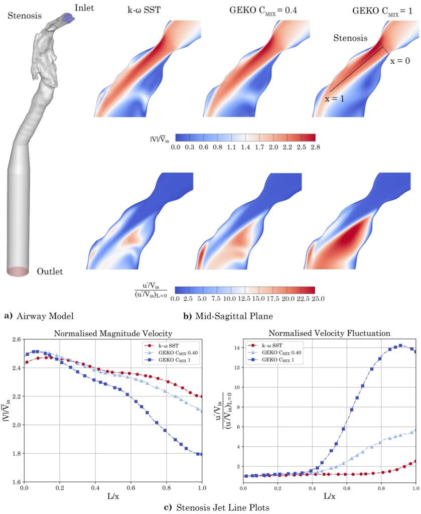
- The article concludes with simulations of flow through a nasal geometry showing the impact of this parameter change on a real biomedical flow.

This model tuning is not limited to biomedical flows but has been applied to many other applications, including examples as diverse as low-speed aerodynamics, cyclones, heat exchangers and turbine combustors [7].
It should be recognised that the model fitting in this study was done using a simplified parametric study but that there is tremendous potential for these workflows to be automated using Ansys OptiSlang to deliver a much more sophisticated approach to tuning the GEKO constants. If whole field data are available from simulation, Fluent-AI+ can determine a local distribution of model constants to fit the data. Beyond that SIM-AI can be trained using multiple (30-100) simulation datasets to produce a model capable of reproducing the entire flow field. Stay tuned for more on this in future blogs!
References
[1] Menter, F., Two-equation eddy-viscosity turbulence models for engineering applications. AIAA J. 32 (8), 1598–1605, (1994).
[2] Menter, F.; Lechner, R.; Matyushenko, A. Best Practice: Generalized k-ω Two-Equation Turbulence Model in ANSYS CFD (GEKO); ANSYS Germany GmbH: Darmstadt, Germany, (2019).
[3] Menter, F., Hüppe, A., Matyushenko, A., Kolmogorov, D., An overview of hybrid RANS–LES models developed for industrial CFD. Appl. Sci. 11, 2459, (2021).
[4] Menter, F.R., Best practice: scale-resolving simulations in Ansys CFD. ANSYS Germany GmbH, (2012).
[5] J. Emmerling, S. Vahaji, D.A.V. Morton, S. Stevanović, D.F. Fletcher and K. Inthavong, Tuned generalised k-ω (GEKO) turbulence model parameters for predicting transitional flow through stenosis geometries of various degrees. Fluids, 10, 168, (2025).
[6] Ahmed, S.A.; Giddens, D.P. Pulsatile poststenotic flow studies with laser Doppler anemometry. J. Biomech. 17, 695–705, (1984).
[7] H. Kutkan, D. Bessette and G. Klavaris, Efficient and reliable CFD strategies for aeroengine combustors. Int. Soc. Air Breathing Engines, 2024.


