
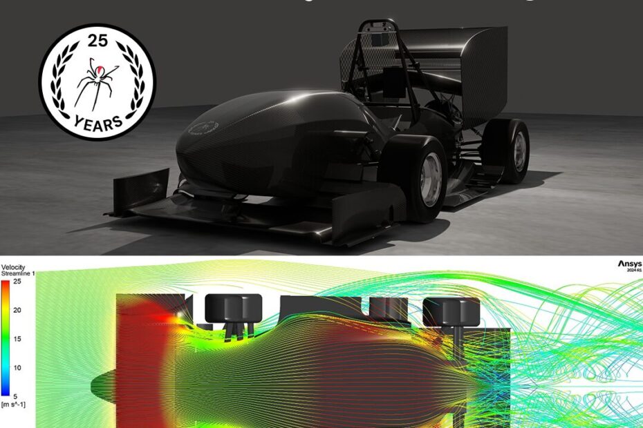
Part 2 – Guest Blog by Julio Martins, former Aerodynamics & Cooling Lead, UNSW Redback Racing
(Revisit Part 1 here – A look back at Redback Racing FSAE Aerodynamics Strategies)
The largest growth in understanding during the design of RB24 came from the characterisation of the package performance in Roll, Pitch, Yaw and Heave as well as analysis of the balance shift with different front and rear wing DRS flap settings. These simulations are what we call “sweeps” as the simulation will sweep through a range of different angles/heights/settings which allows for performance curves to be plotted with respect to the variable being analysed. This is where I began to look beyond the usual visual contour results typical of CFD and more into the numbers and underlying relationships. Rather than analysing each design point in isolation, they were plotted and analysed wholistically for all the design points to better understand how the downforce, drag and balance all varied across each separate component and the whole car. These plots then allowed us to see how the package behaves in all different cases, both within and outside of its expected handling envelope, and what effect the package will have on the vehicle dynamics. This grew our understanding of the package behaviour which we could then go and relate back to the individual design points of interest to determine why a certain phenomenon is occurring (front wing stall at high nose down pitch for example).
Below I will go through some of the more condensed charts which I produced. They show the downforce and aerodynamic balance variation on a single chart for the full car and each separate component. Similar graphs were plotted for drag as well but are not shown here. Later I will show some other graphs plotted from the Yaw simulation which provide very useful insights into the vehicle dynamics interaction of the package and show the usefulness of the less common results to analyse within a simulation of an FSAE car.
One important aspect to note is that in all the characterisation simulations, the variable range simulated was based on a physical limitation rather than a kinematic limitation of the suspension. It was calculated that the maximum pitch angle under braking with our kinematics setup would be 0.5 degrees, however the aerodynamics package was simulated up to 1.2 degrees in pitch. Why 1.2 degrees? Because that’s the pitch angle when the front wing hits the ground. In the same way, roll was simulated up to 1.8 degrees which is when the undertray footplate would hit the ground. This allowed us to determine the absolute dynamic limit of the aerodynamics package and determine the behaviour outside of its handling envelope if the kinematics setup was ever to change. It therefore allowed us to determine the limits of our design. The expected handling envelope is indicated within a dashed box on each graph.
For clarity, the aerodynamic balance by convention is given as the percentage of the total downforce acting on the front wheels. A balance of 52% will therefore have more front downforce than a balance of 48%. The aerodynamic balance is a result of the longitudinal location of the centre of pressure (CoP) between the front and rear wheels. Its lateral location also influences lateral balance which I will touch on later.
Roll Results
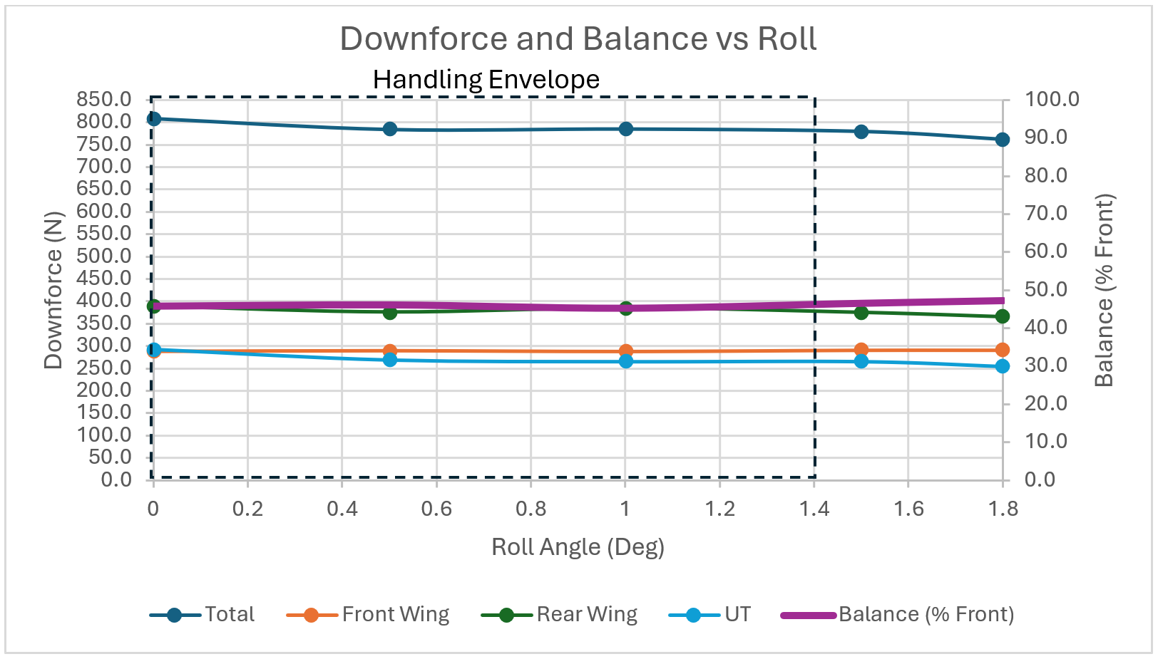
It can be seen from the graphs of downforce and balance vs roll angle above that the aerodynamic balance of the car does not shift substantially during roll, remaining steady around 47% front balance. It can also be seen that the downforce across the full package and each component remains consistent with no sudden change (especially within the handling envelope of 0 to 1.4 degrees). This is ideal for us as it means the driver will not experience any sudden change in balance or downforce as the car rolls, providing them with a predictable and stable platform.
Pitch Results
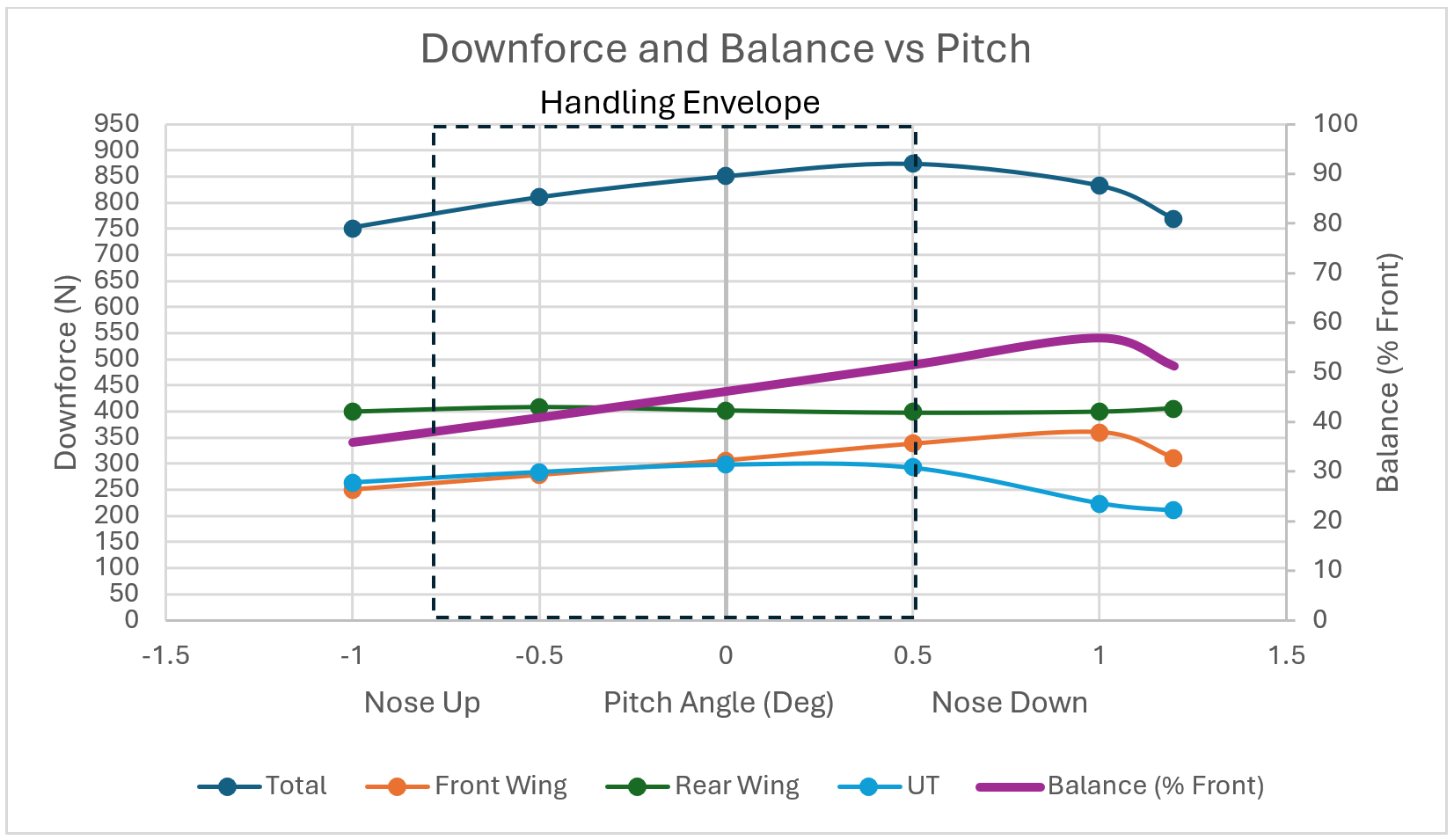
Moving to the pitch results, this is where to begin to see some more interesting and complex package behaviour with more variation. More variation is not always a bad thing and is often desired if it varies favourably.
Looking at the balance variation first, we can see that at 0 degrees of pitch, the balance is at 47% just like in the roll case. As the car pitches nose down (positive) which would be associated with a braking case into a corner, we can see that the balance begins to shift forward and provide more aerodynamic load onto the front tyres. The balance shift peaks at 57% at 1 degree before retreating backwards at 1.2 degrees because the front wing begins to stall due to ground contact. This forward shift of the aerodynamic balance is desirable as it means more aerodynamic load is applied to the front tyres during braking which improves braking performance. The forward balance under braking also means that the front tyres will experience more grip on corner entry thus reducing understeer on corner entry. The drop in aerodynamic balance at high pitch angle (>1 degree) is not desirable however given the maximum normal pitch angle is 0.5 degrees, the car would usually never get to the point of the balance shifting backwards and so it not a concern. During acceleration, we can see the balance shifting rearwards as the nose lifts and the rear squats. This backwards shift in balance is also desirable as it moves the centre of pressure rearwards, further behind the centre of gravity of the car which helps improve stability during acceleration, reducing the likelihood of corner exit oversteer. This also places more aerodynamic load on the rear (driven) tyres, improving grip and reducing wheel spin during acceleration. This is an example of a desirable shift in balance which is beneficial to the vehicle dynamics of the car.
Furthermore, it can also be seen that the total package downforce reaches a maximum at 0.5 degrees nose down pitch. This therefore means that coupled with the forward balance shift, the package also generates the most downforce when under maximum braking, helping push the car into the track to maximise braking performance. We can also see that at nose down pitch angles greater than 0.5, the downforce of the package begins to drop as certain components begin to lose capacity to generate maximum downforce. This begins with the undertray loosing performance as the front wing becomes closer to the ground, removing more energy from the flow entering the floor. This loss then shifts to the front wing at nose down pitch angles greater than 1 degree as the front wing begins to stall and choke, further reducing the undertray performance. The rear wing performance however remains consistent as expected. In nose up pitch conditions, we can see the downforce gradually reduce as all the wings have a lower effective angle of attack which is expected and has a small drag reduction which is beneficial to acceleration performance.
Heave Results (Ride Height Change)
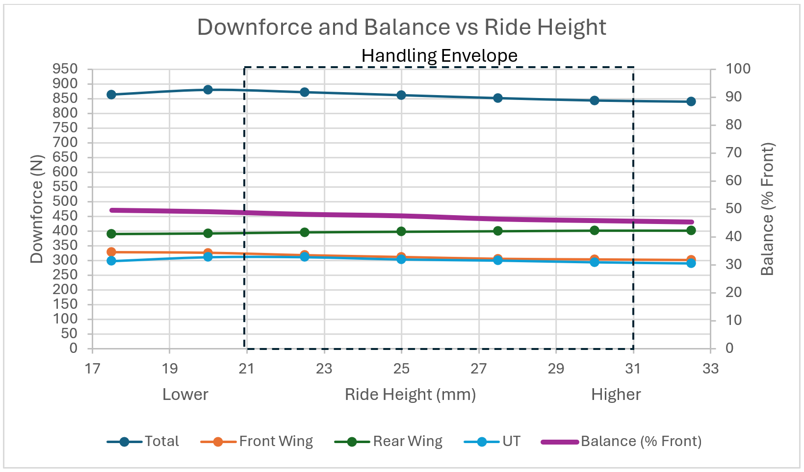
Now looking at the heave simulation, the balance remains linear with a slight forward shift as the ride height decreases. The reason for this shift is that the downforce generation of the front wing and undertray increases as the ride height decreases which tends to move the balance forward. The balance therefore shifts forward linearly from 45% to 50% as the ride height decreases from 32.5mm to 17.5mm.
The total package downforce also increases as the ride height decreases for the same reason as the balance shift above. The graph shows that there is no sudden change in balance or downforce across ride height which is desirable. Any sudden losses across the ride height sweep would be an indication of component (undertray) stall which could likely result in a phenomenon known as “porpoising” which has been an issue for some Formula 1 teams during the 2022 to 2025 regulation period.
Yaw Results
The Yaw characterisation is the most important and useful simulation for us as our cars spend majority of their time on track in a yaw case. It is also the case where cars can be most sensitive and show the largest variations in balance and downforce and the case to which the aerodynamics is most sensitive. Designing for yaw stability is difficult as it not only results in a longitudinal balance shift like roll, pitch and heave, but it also causes a shift in lateral balance which poses several dynamic challenges.
Before diving in however, it is important to be aware of the simulation setup and its compromises as not all yaw simulations are the same. The yaw simulation performed made use of what is known as a “D-domain” where the inlet and ground velocity vectors are parameterised to produce the desired yaw angle by varying the U and V (longitudinal and lateral) velocity magnitudes to change the direction of the airflow and ground through the domain.
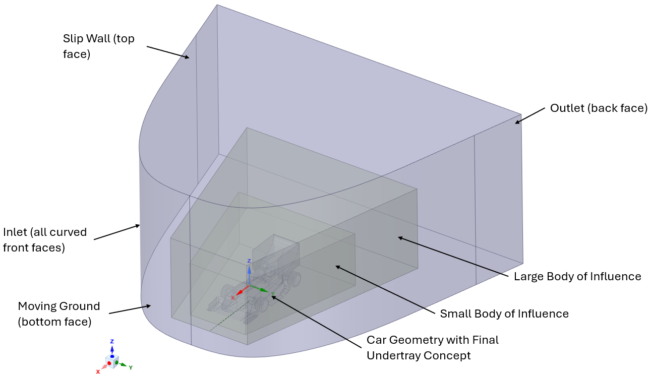
This means however that the full vehicle and all the aerodynamics components will see the same yaw angle. This is different to a cornering type simulation where a curved domain is used to simulate a corner of a specific radius. A cornering simulation will result in the rear wing seeing a smaller yaw angle than the front wing as opposed to the same yaw angle across the entire car as is the case with the simulation we performed. This will result in larger total package losses for our simulation setup compared to an equivalent cornering type simulation however it greatly reduces setup and computation time by allowing a single geometry to be used with the inlet and ground velocity parameterised directly in Ansys Workbench. The one drawback is that by using the same geometry, the front wheels cannot be turned as the yaw angle changes which does influence the results. I believe the results from a “D-domain” type yaw simulation are more conservative than a cornering type yaw simulation and it also allows for analysis of oversteer cases which would require a different setup in a cornering type simulation.
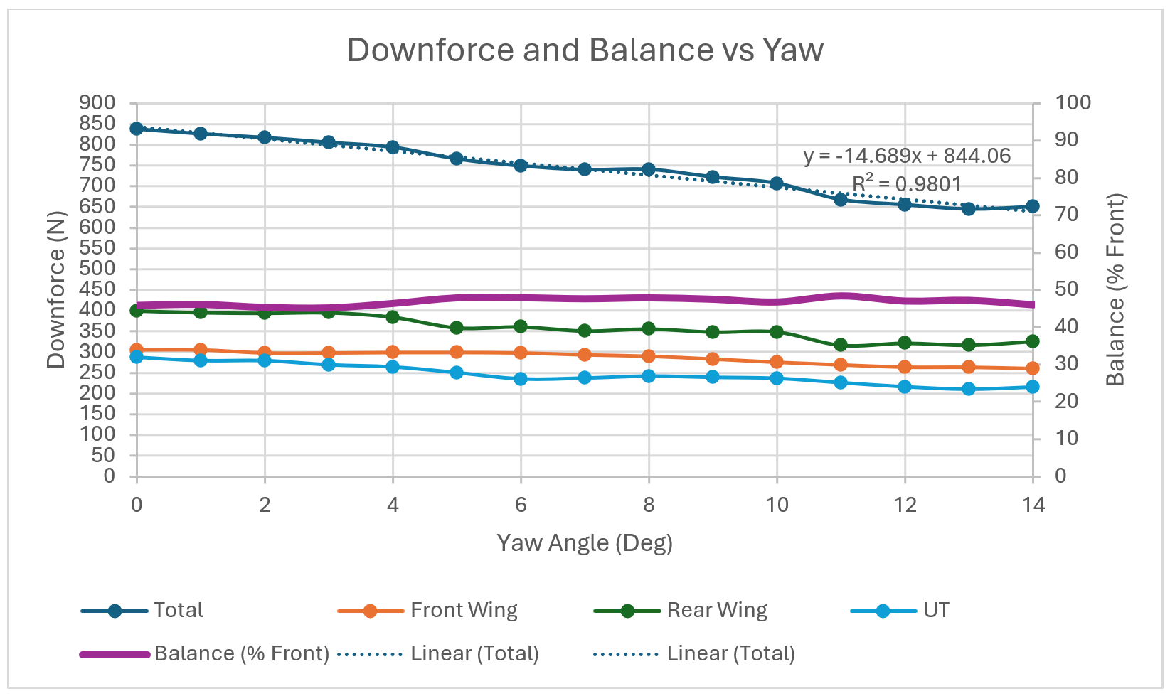
We can see from the graph of downforce and balance vs yaw angle that the longitudinal balance tends to oscillate between 45% and 48% as the yaw angle changes from 0 degrees to 14 degrees. This oscillation is small enough that its noticeability to the driver is minimal and has a very small effect on the vehicle dynamics. I will come back to the balance shift later looking at more precise metrics.
Looking at the downforce for the full package and each of the components, we can tell which components are more greatly affected by yaw. The total package downforce decreases almost linearly up to 22% as the yaw angle increases from 0 to 14 degrees. Although this reduction in downforce itself is not completely favourable, the linear and relatively low (±20%) decrease in total downforce is favourable compared to a sudden large drop in downforce at a lower yaw angle. In fact, when plotting a line of best fit on the total downforce graph, the gradient shows that for a yaw angle of 0 to 14 degrees the package loses around 15N of downforce per degree of yaw (15N /deg).
The graph also shows that the rear wing and undertray are more affected by yaw than the front wing which also explains the slightly forward shift in longitudinal balance at higher yaw angles. Overall, it was concluded that the package performance in yaw was sufficiently stable to provide a predictable platform for the driver to rely upon with no sudden losses or changes in balance.
With the overall downforce and balance analysis completed, we can move into the less common characteristics of the package in yaw and the detail that CFD simulation is able to provide to improve understanding of the package behaviour.
Corrective Torque
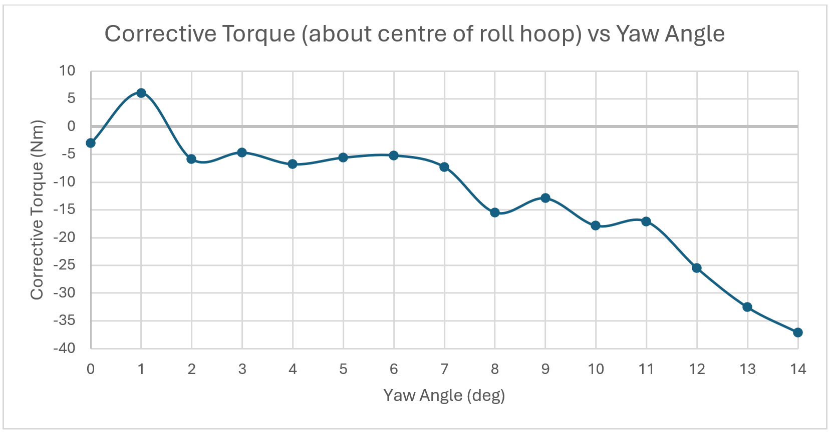
The graph above shows the corrective torque about the roll hoop of RB24 as yaw angle increases. The reason for this corrective torque is because of the rear wing endplates working to correct the cars motion in the case of oversteer just like the feathers on the back of a dart. The graph above quantifies the torque produced by the rear wing endplates as the vehicles yaw angle increases.
Lateral Force
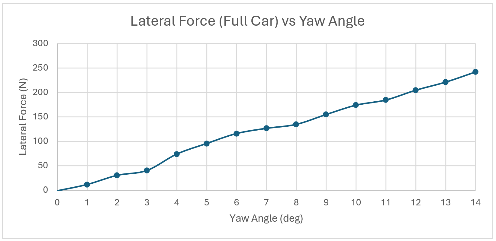
The graph above is less commonly shown when analysing the aerodynamic performance of a car but shows the lateral force generated because of increasing yaw angle. When there is no yaw angle, the lateral force is zero but as the yaw angle increases, more of the airflow is incident on the side of the car, therefore generating a lateral force. In a steady state cornering scenario with no slip, this lateral force tends to push the car outwards of the corner, which is undesirable. However, the median yaw angle of the car in steady state cornering tends to only be around 2 degrees which results in very low lateral force pushing the car out of the corner. Where this graph becomes interesting is when considering an oversteering case in which the full car will see a much larger yaw angle across all components. This graph is ideal for analysing this case and shows that in a case of 14 degrees of oversteer, there will be nearly 250N of force pushing the car into the corner and working to reduce the lateral (outward) slip of the oversteer which is desirable.
In my opinion, the most fascinating results determined from the yaw simulation were the graphs plotted below. These graphs plot the physical change in position of the Centre of Pressure (CoP) of the package as the yaw angle changes. The position change is measured relative to the position of the CoP at zero degrees of Yaw.
Longitudinal CoP Shift
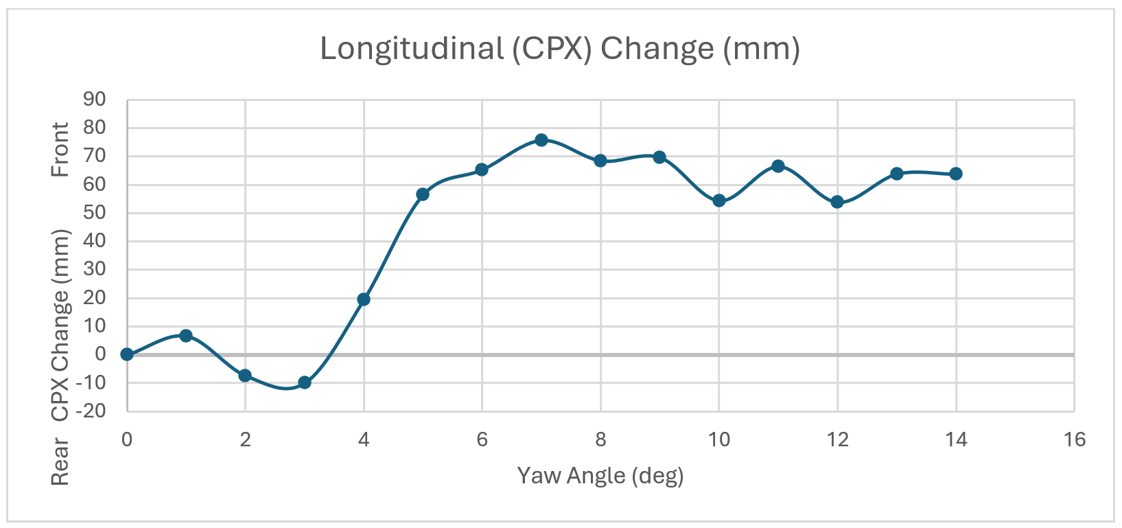
The graph above plots the change in the longitudinal position of the centre of pressure as the yaw angle increases. For low yaw angles, the longitudinal shift oscillates between ±10mm from 0 to 3 degrees after which the CoP shifts forward as shown in the Downforce and Balance vs Yaw graph earlier. The above graph does provide more detail in the magnitude of the CoP shift and the oscillations of the CoP location between 6 and 14 degrees. Despite the oscillations, it shows an overall forward shift in CoP of around 60mm at higher yaw angles.
Lateral CoP Shift
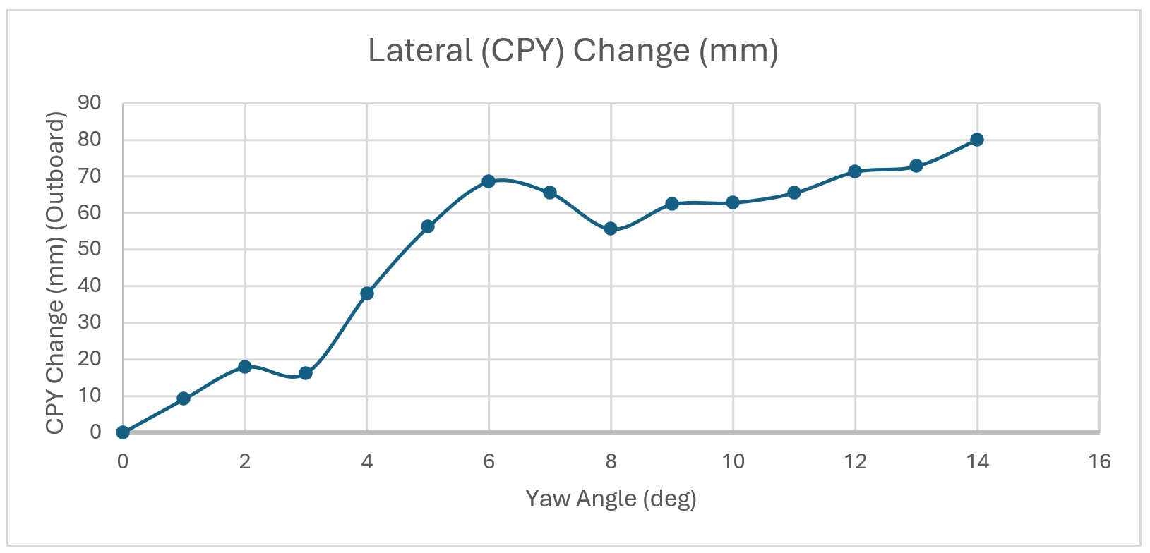
The graph above shows the lateral position change of the centre of pressure as the yaw angle increases. The lateral centre of pressure location begins on the centreline plane of the car and shifts outboard as the yaw angle increases. The CoP shifts back towards the centreline plane between 6 and 8 degrees and then begins to move outboard again. The total lateral outboard shift is 80mm which is quite a small lateral shift given the 1250mm track width of the car. Keeping the lateral CoP shift as low as possible is desirable as it maintains a more even aerodynamic load balance between the inboard and outboard tyres of the car while cornering. This avoids applying too much aerodynamic load to the outboard tyres during cornering which are already heavily loaded due to mechanical load transfer. Keeping the lateral CoP central improves cornering performance by keeping the outside tyres further away from critical tyre load sensitivity.
DRS Characterisation
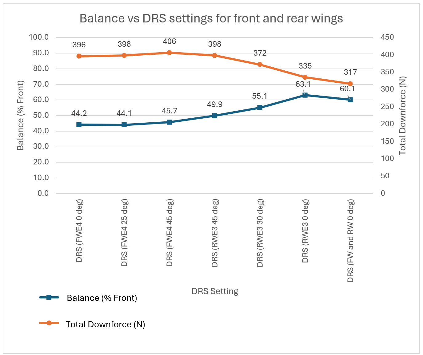
We also characterised the downforce and balance changes with different front and rear wing DRS settings for testing purposes. This allowed us to perform on track testing with different longitudinal aerodynamic balances to determine the effect of moving aerodynamic balance on vehicle handling and driver preferences to better determine aerodynamic targets for 2025. The graph above shows the aerodynamic balance and total vehicle downforce for changing DRS settings from front wing fully open (left) to closed through to rear wing fully open and then finally both front and rear fully open. This shows that we have a 20% balance shift bandwidth available for testing using a range of DRS settings which is beneficial to further growing understanding of the package dynamics.
Stay tuned for Part 3 in this series where Julio focuses on visualisation of aerodynamics flow structures and overall flow “cleanliness” with comparisons between RB23 and RB24.